Dear Brian, 

So, I hear you’re the data expert? Well, I’ve got a conundrum for you. As an RA for SpokenWeb, we’re often working with disorganized, unlabelled, and sometimes incomplete archival collections. Take, for instance, the Alan Lord Collection we are currently working on. For context, this collection includes AV materials from Ultimatum [1] and Ultimatum II, punk poetry music festivals that Alan organized in the 80s, in Montreal, at the iconic Foufounes Électriques. The festivals featured poetry readings, musical performance, computer art, and electronic sounds, all in a distinctly punk experimental flavor.  The AV assets for this collection presented a particular challenge: the audio materials came to us recorded on multitrack tapes. That is, each tape had eight different tracks running parallel to each other. When we had the tapes digitized, each of the eight tracks from a single tape was bounced (outputted) as its own individual digital audio file.  So one reel to reel multitrack tape generated eight WAV files. There might be a kick drum pounding for a while on one track, a voice reciting poetry on another, a keyboard riff on another, etc. Sometimes all eight tracks on the tape were used to record the sounds of a single event. Sometimes, if less tracks were needed, two different events were recorded parallel to each other (for example, one event on tracks 1-4, another event on tracks 5-8). As you can imagine, this has resulted in a sense of total chaos as we approach our numerous audio files and try to link them up to the correct performances so we can mix them down into a full audio recoding of each event as it sounded.

Attending to these multitrack tapes with the goal of reconstructing the full sonic image of different events has required careful listening to individual tracks, research, and a fair amount of guessing. Some tracks contain audio for two, or three different performances (one after another)! Silence, applause, and notes from Alan have helped guide our listening, but I wonder whether this listening work could be streamlined.

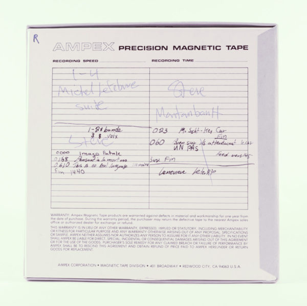
One of the reel-to-reel tape boxes from the Alan Lord collection, with basic information about track contents.

So, my question for you is: would there be a way to automate this process of identifying which individual tracks were documenting the same event? That is, could you design an algorithm to figure out, without having to listen to countless hours of audio, which of the multiple tracks belong together? Could a computer automatically remix these, and reconstruct the original sets, before having the human listen? In sum, could an algorithm be designed to automatically mix and match multitrack recordings of numerous distinct poetry and music events, so that the correct individual tracks are clustered together?

Signed,    

All Mixed Up

Dear All Mixed Up, 

This question is an interesting puzzle, and I mean that in the most literal sense.  The problem you describe is in some sense the audio equivalent of a jigsaw puzzle: you have a collection of pieces that need to be reassembled into their original coherent order. Computer scientists love this kind of thing, and I’ve even spent quite a bit of time in my own research working on related problems that show up in music playlist composition and audio representation learning. 

The bad news is that we probably can’t come up with a magical algorithm that will solve this problem for you entirely.  The good news is that we can still use computers and audio analysis to reduce the amount of effort it would take a person to reassemble the clip sequence!   

Looking around my audio collections, I didn’t have anything lying around that naturally fit your problem description.  However, the Internet Archive has a huge collection of audio resources that could be used to simulate your problem setting. In particular, their Grateful Dead  repository contains thousands of concert recordings, which have been digitized and separated into individual songs.  For the purposes of this column, I downloaded one concert (1994-10-19 at Madison Square Garden), which consists of 20 tracks recorded over three digital audio tapes.  If we ignore the metadata (track title, tape number, sequence number), then we have a reasonable approximation to your clip sequencing problem. 

Now that we have a collection of recordings, the key thing to observe is that the end of one recording should sound “similar” to the beginning of the next recording when the tracks are properly sequenced. Think of this as the acoustic equivalent of two jigsaw pieces fitting together. If we can uniquely identify which ends and beginnings match up to each other, then our problem becomes much simpler! 

 In my previous column, I showed how we can use spectrograms to visually identify features of different kinds of applause.  We can do a similar trick here, except now we’re looking to match fragments of audio to each other instead of identifying their exact contents.  For example, if we were to compare the last second of audio from one track (the query) to the first second of audio from the beginning of each other track, we’d get something like the following: 

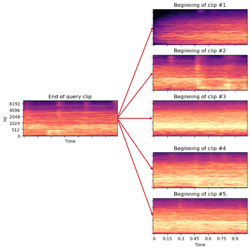
For each of these images, the color represents how much energy is present at each frequency (vertical axis) over time (horizontal axis).  To a layperson, these images probably all look quite similar to each other, but an expert could probably determine with reasonably high confidence that the second clip is the best match to the query, based on the general distribution of energy across frequencies and periodic vertical structures common to both. 

If you don’t happen to have an expert audio analyst lurking around, we can ask a computer to do this for us instead.  A typical approach to this would be to treat each vertical column of the spectrogram image as a representation of the audio at a particular point in time.  If we then compare each of these time-points to each other time-point in our collection, we can build up a “distance matrix” as shown here: 

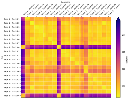
In this image, each row corresponds to a short fragment from the end of a recording, and each column corresponds to a fragment from the beginning of a recording.  Bright colors indicate high similarity (small “distance”), and dark colors indicate low similarity (large distance).  I’ve organized the image here according to the true identities of the tracks in question (in the correct order), and from each recording I’ve taken five spectrogram columns, which is equivalent to about 1/10th of a second. If this was working properly, we would see bright colors down the northwest-southeast diagonal, meaning that track 1 leads into track 2, track 2 into track 3, and so on, and dark colors off the diagonal, indicating that track 1 does not lead into track 3, for instance.  The astute reader will notice at this point that this approach did not work at all: everything looks basically similar to everything else! 

Let’s not give up just yet.  There is still some information that we haven’t used.  In the distance matrix illustrated above, I’ve drawn lines between each track to help guide the eye.  While we don’t really know the identity and sequence order of each track, we do at least know which track produced each spectrogram.  If we can somehow transform our representation of audio so that all data coming from the beginning of a track are closer to each other than they are to the beginning of other tracks, we should get some more discriminative power out of our approach. 

Luckily for us, there are dozens of methods for this exact problem.  The one I’ll use here is called UMAP (Universal Manifold Approximation), which sounds fancy—and it is!  At a high level, what this method can do is learn a mapping from a high-dimensional space—in our case, hundreds of dimensions corresponding to different frequencies—into a low-dimensional space (e.g., 2 or 3).  We can also tell UMAP which data points “belong together” and which ones do not.  In our case, we’ll use only the data from the beginning of each recording, and tell UMAP to keep each recording separate from all the others.  Note that we don’t need to know the true name or ordering of the recordings here, it’s enough to give each recording its own pseudonym here. 

After UMAP does its job, we can apply the learned transformation to both the beginning fragments and the end fragments, and then compute distances just like we did before.  The result will look something like this: 

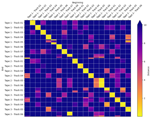
Clearly, this is still not perfect, but we do have something much closer to usable!  As we had initially hoped, there is now indeed a bright yellow strike down the main diagonal, indicating that most of the time, the ending of one track is correctly matched to the beginning of the next track.  There are of course also some mistakes: Tape 1 – Track 08 matches mostly to Tape 2 – Track 01 (correct), but also a little to Tape 1 – Track 01.  As long as the mistakes are in the minority, this will not hurt us.  A more serious mistake occurs at the end of Tape 3 – Track 06 (bottom row), which is the final track in the recording.  Of course, the distance calculation above doesn’t know this to begin with, so it tries its best to find a match, which in this case is the beginning of Tape 2.  These mistakes are all reasonable given the nature of the data – tape transitions align with set transitions during the concert, which will have similar patterns of fade-in/fade-out and crowd noise.  In fact, the only serious mistake made here is that Tape 2 – Track 05 matches more highly to Tape 3 – Track 01 than to its true successor (Tape 2 – Track 06). 

 Okay, so what do I do with all of this?   

With the distance matrix computed above, we can compare the end of each track to the beginning of each other track.  When we see a pair that has much smaller distances than the rest, we can determine that these two probably should go in order.  There will of course be mistakes and ambiguities in this process, and we won’t be able to definitively tell which track comes first.  However, we have vastly simplified the problem by ruling out the majority of sequence decisions that are likely to be obviously wrong.  At this point, the remaining work to resolve mistakes and ambiguities could be accomplished reasonably quickly by an astute listener such as yourself! 

In many cases, this is where computational audio analysis fits best.  Machines are not likely to solve everything for us, but with a little effort and know-how, they can at least help with the boring parts so that we can focus on the more fun activities. 

Brian